The FILTER function in Google Sheets: 7 examples

Q: Can FILTER return only some columns?

Yes. Use a narrower range: =FILTER(A2:A9, C2:C9>=40) returns only the names.

Q: How do I filter by part of a word?

Use SEARCH: =FILTER(A2:E9, ISNUMBER(SEARCH("sh", D2:D9))) finds every item containing “sh”.

1 Oct 2026 · 4 min readFILTERGoogle SheetsExcel 365

Before/after: the full table on the left, the filtered list on the right, the formula in between

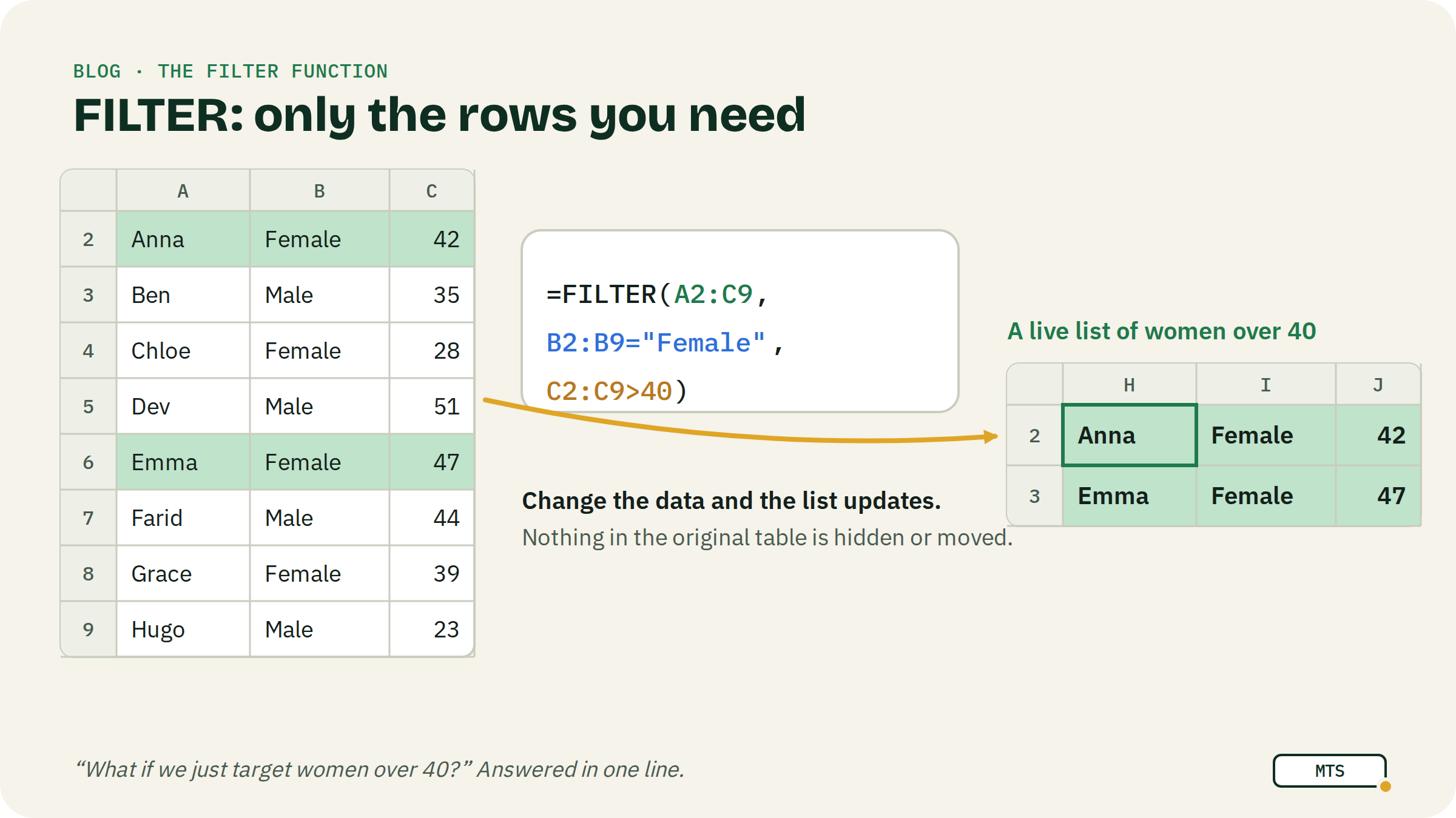
FILTER returns only the rows that meet your conditions, as a live list that updates when the data changes: =FILTER(range, condition). Unlike the filter button, it doesn't hide anything. It builds a new list you can put anywhere.

If you've ever worked with a dataset of more than 100 rows, you probably get the point: life would hit different without filters.

I remember the first time I sat in a meeting with senior stakeholders over my broken financial model. They asked questions like “what about this cohort?”, “what about prices over X?”, “what if we just target women over 40?”. Every question meant scrolling, clicking and hoping.

If you want to avoid the heavy breathing in a situation like this, pay attention to the examples below. They all use the same small table.

	A: Name	B: Gender	C: Age	D: Item	E: Price
2	Anna	Female	42	Bag	120
3	Ben	Male	35	Shoes	85
4	Chloe	Female	28	Scarf	25
5	Dev	Male	51	Watch	240
6	Emma	Female	47	Shoes	95
7	Farid	Male	44	Bag	60
8	Grace	Female	39	Scarf	30
9	Hugo	Male	23	Shoes	70

How FILTER works

=FILTER(range, condition1, [condition2, …])

range: the rows you want back, e.g. A2:E9.
condition: a column compared to something, e.g. B2:B9="Female". Same number of rows as the range.
Write it in one empty cell. The results spill down and right, so leave room.

1. Filter by gender

=FILTER(A2:E9, B2:B9="Female")

Returns Anna, Chloe, Emma and Grace, with all five columns.

2. Filter by age

=FILTER(A2:E9, C2:C9>=40)

Returns Anna (42), Dev (51), Emma (47) and Farid (44). Numbers need no quotes.

3. Items over X

=FILTER(A2:E9, E2:E9>80)

Returns Anna, Ben, Dev and Emma. Better: put the 80 in a cell (say H1) and write E2:E9>H1. Now anyone in the meeting can change the number and watch the list update. This is the answer to “what about prices over X?”.

4. Items under X (and what to do when nothing matches)

=FILTER(A2:E9, E2:E9<50)

Returns Chloe (25) and Grace (30). If nothing matches, FILTER shows an #N/A error. Wrap it to show a friendly message instead:

=IFERROR(FILTER(A2:E9, E2:E9<20), "Nothing under 20")

5. Combine conditions (AND): women over 40

In Google Sheets, just add more conditions, separated by commas. A row must pass all of them:

=FILTER(A2:E9, B2:B9="Female", C2:C9>40)

Returns Anna and Emma. That's the stakeholder question, answered in one line.

6. Either/or (OR): shoes or bags

For OR, put each condition in brackets and add them with +:

=FILTER(A2:E9, (D2:D9="Shoes")+(D2:D9="Bag"))

Returns Anna, Ben, Emma, Farid and Hugo. The rule to remember: * between conditions means AND, + means OR.

7. Filter, then summarise (a mini pivot)

FILTER gets even more useful inside other formulas. How much did women over 40 spend, and how many of them are there?

=SUM(FILTER(E2:E9, B2:B9="Female", C2:C9>40))        → 215
=COUNTA(FILTER(A2:A9, B2:B9="Female", C2:C9>40))     → 2
=SORT(FILTER(A2:E9, C2:C9>=40), 5, FALSE)           → over-40s, most expensive first

This is how you answer pivot-table questions without a pivot table. (To filter an actual pivot table, use its own filter or a slicer. FILTER works on the source data.)

FILTER in Excel

Excel has FILTER too (Microsoft 365 and Excel 2021 or newer), with two differences:

Only one condition argument. Combine conditions inside it: =FILTER(A2:E9, (B2:B9="Female")*(C2:C9>40)).
A built-in “if empty” argument, so you don't need IFERROR: =FILTER(A2:E9, E2:E9<20, "Nothing under 20").

Two Excel differences: SORT takes 1 or -1 for the order (write =SORT(FILTER(...), 5, -1), not FALSE), and Excel's FILTER takes only one include argument, so combine conditions with * (AND) or + (OR): =FILTER(A2:E9, (B2:B9="Female")*(C2:C9>40)). When nothing matches, Excel shows #CALC! instead of #N/A.

Common mistakes

#REF! instead of results (#SPILL! in Excel). Something is in the way of the spill. Clear the cells below and to the right.
Different sizes. A2:E9 with B2:B20 fails. The condition must cover the same rows as the range.
Text without quotes. B2:B9=Female doesn't work. Write "Female".
Typing over the results. You can't edit a filtered result cell. Change the source data or the condition instead.

FAQ

What's the difference between FILTER and the filter button? The button hides rows in the original table. FILTER builds a separate, live list and leaves the original untouched.

Can FILTER return only some columns? Yes. Use a narrower range: =FILTER(A2:A9, C2:C9>=40) returns only the names.

Does the result update automatically? Yes. Change a price or add a row inside the range, and the list updates.

How do I filter by part of a word? Use SEARCH: =FILTER(A2:E9, ISNUMBER(SEARCH("sh", D2:D9))) finds every item containing “sh”.

Keep going

Next read: SUMIFS explained with 5 real examples. It's the other half of the “what about X?” toolkit.
Practise sorting and filtering in White Belt lesson 12.

Written by MasterTheSheets