SUMIFS explained with 5 real examples
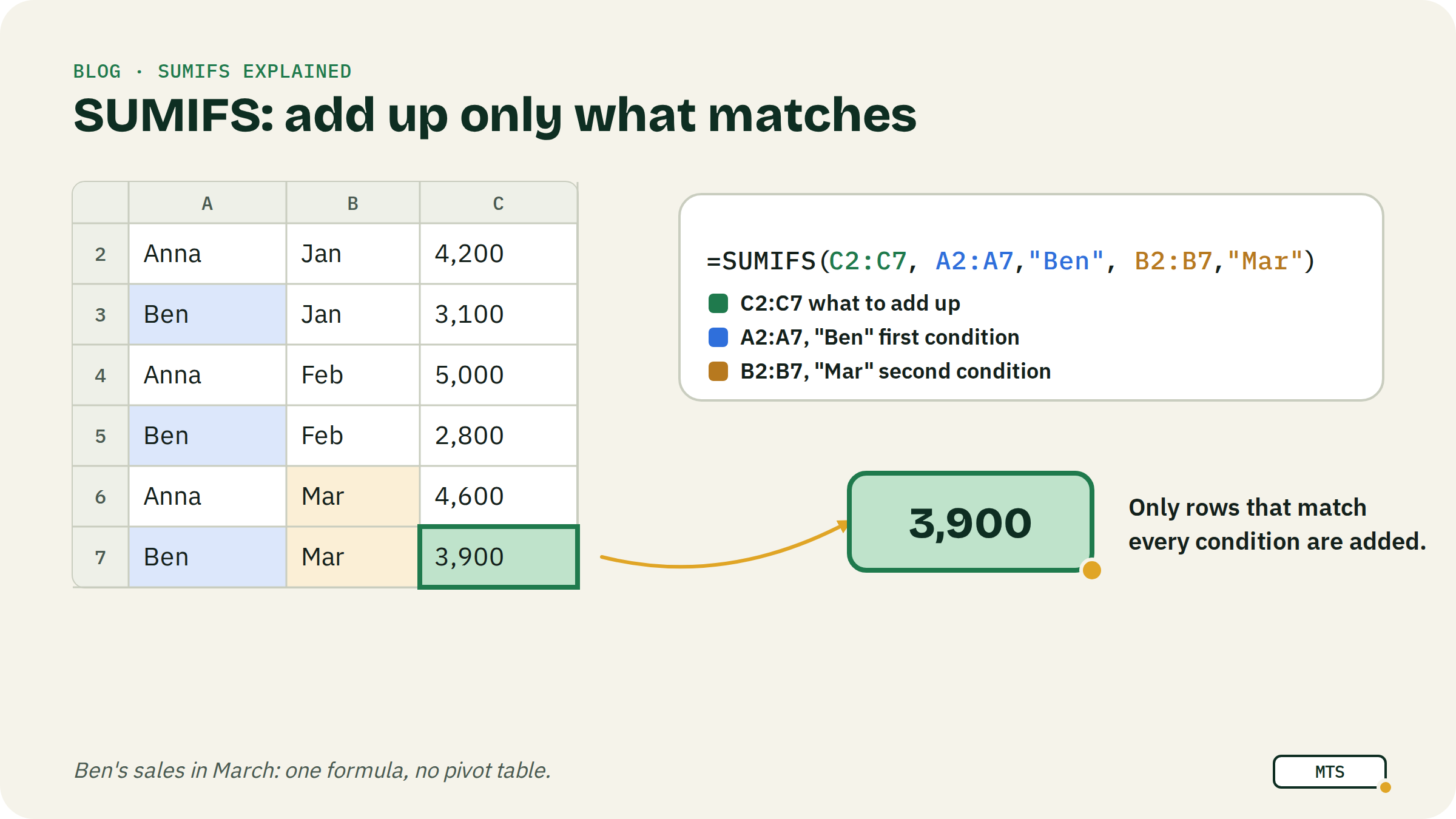
SUMIFS adds up only the numbers that match your conditions: =SUMIFS(what to add, where to look, what to match, …). It answers “how much did X make?” in one cell, without building a pivot table.
It is strange to write, but one of the most underrated formulas is SUMIF, and its bigger version, SUMIFS.
SUM is something a smart eight-year-old can learn. Now meet the cool older brother of SUM.
If you don't want to complicate things with a pivot table and just want to see quickly how your sales team performed this month, SUMIFS is the way to go. (And if you want to count instead of add, like how many students in your class reached a 3.5 GPA, its sibling COUNTIFS works exactly the same way.)
How SUMIFS works
=SUMIFS(sum_range, criteria_range1, criteria1, [criteria_range2, criteria2], …)- sum_range: the numbers you want to add up (e.g. the Sales column).
- criteria_range1: where to look (e.g. the Name column).
- criteria1: what to match (e.g. "Anna").
- Add more pairs of where to look + what to match for every extra condition. A row is only added if it matches all of them.
SUMIF (without the S) takes only one condition, and the order is different: =SUMIF(where to look, what to match, what to add). If you learn only one, learn SUMIFS: it handles one condition too.
1. Team performance: who sold what, and when
You track your team's sales in a sheet with monthly data. After the third month things get noisy, and you can't catch trends in a fraction of a second anymore.
| A: Rep | B: Month | C: Sales | |
|---|---|---|---|
| 2 | Anna | Jan | 4,200 |
| 3 | Ben | Jan | 3,100 |
| 4 | Anna | Feb | 5,000 |
| 5 | Ben | Feb | 2,800 |
| 6 | Anna | Mar | 4,600 |
| 7 | Ben | Mar | 3,900 |
Anna's total so far:
=SUMIFS(C2:C7, A2:A7, "Anna") → 13,800Ben in March only (two conditions):
=SUMIFS(C2:C7, A2:A7, "Ben", B2:B7, "Mar") → 3,900Pro move: type the rep's name in a cell (say F2) and point at it: =SUMIFS($C$2:$C$7, $A$2:$A$7, F2). Fill it down next to a list of names and you have a leaderboard that updates itself.
2. A small bakery: what actually sells
You run a small bakery and want to know your best-selling categories: pastries, milk, soft drinks.
| A: Product | B: Category | C: Revenue this week | |
|---|---|---|---|
| 2 | Croissant | Pastries | 420 |
| 3 | Cinnamon roll | Pastries | 360 |
| 4 | Fresh milk | Milk | 150 |
| 5 | Chocolate milk | Milk | 90 |
| 6 | Lemonade | Soft drinks | 210 |
| 7 | Cola | Soft drinks | 130 |
=SUMIFS(C2:C7, B2:B7, "Pastries") → 780Put the three category names in E2:E4, write =SUMIFS($C$2:$C$7, $B$2:$B$7, E2) in F2 and fill down: Pastries 780, Soft drinks 340, Milk 240. That's a mini report in three cells.
3. Your own spending: how much went on coffee last month?
Do you track your spending? Then check how much you spent on coffee last month. This is where dates come in.
| A: Date | B: Category | C: Amount | |
|---|---|---|---|
| 2 | 28 Aug 2026 | Coffee | 3.80 |
| 3 | 2 Sep 2026 | Coffee | 4.20 |
| 4 | 5 Sep 2026 | Groceries | 46.10 |
| 5 | 9 Sep 2026 | Coffee | 3.80 |
| 6 | 17 Sep 2026 | Coffee | 4.50 |
| 7 | 1 Oct 2026 | Coffee | 4.20 |
Coffee in September only:
=SUMIFS(C2:C7, B2:B7, "Coffee", A2:A7, ">="&DATE(2026,9,1), A2:A7, "<"&DATE(2026,10,1)) → 12.50The date conditions are just two more pairs: on or after 1 September, and before 1 October. Note the ">="& part: the comparison goes in quotes and is glued to the date with &.
4. Travel costs: who paid for what
A weekend away with friends, one shared sheet, and the eternal question at the end: who owes whom?
| A: Who paid | B: Category | C: Amount | |
|---|---|---|---|
| 2 | Priya | Stay | 480 |
| 3 | Tomás | Food | 64 |
| 4 | Aiko | Transport | 36 |
| 5 | Priya | Food | 112 |
| 6 | Sam | Fun | 150 |
| 7 | Tomás | Food | 18 |
=SUMIFS(C2:C7, A2:A7, "Priya")                      → 592   (everything Priya paid)
=SUMIFS(C2:C7, B2:B7, "Food")                       → 194   (the whole food bill)
=SUMIFS(C2:C7, A2:A7, "Priya", B2:B7, "Food")       → 112   (Priya's food only)
Total the trip, divide by four, and compare with each person's SUMIFS: that's your settle-up list.
5. Screen time check
Export your screen time (or just jot it down for a week) and ask the uncomfortable question: how much time goes on social apps on work days?
| A: Day | B: App | C: Type | D: Minutes | |
|---|---|---|---|---|
| 2 | Mon | Social | 48 | |
| 3 | Mon | Duolingo | Learning | 15 |
| 4 | Tue | TikTok | Social | 62 |
| 5 | Tue | Social | 30 | |
| 6 | Sat | TikTok | Social | 95 |
| 7 | Sun | Social | 70 |
=SUMIFS(D2:D7, C2:C7, "Social", A2:A7, "<>Sat", A2:A7, "<>Sun") → 140 minutes"<>Sat" means “not Saturday”. You can use the same column twice, once for each day you want to leave out.
Common mistakes
- Ranges of different sizes.
C2:C7withA2:A10gives an error (#VALUE! in Google Sheets). Every range must have the same number of rows. - Mixing up SUMIF and SUMIFS. SUMIF puts what to add last, SUMIFS puts it first.
- Comparisons without quotes. Write
">100", not>100. Pointing at a cell?">"&F1. - Numbers stored as text. If a total looks too small, check that the amounts are real numbers (right-aligned) and not text.
- Expecting OR. SUMIFS only does AND: every condition must be true. For “Coffee OR Tea”, add two SUMIFS together.
FAQ
What's the difference between SUMIF and SUMIFS? SUMIF takes one condition, SUMIFS takes one or more, and the argument order is different. SUMIFS can do everything SUMIF does.
Does SUMIFS work the same in Excel and Google Sheets? Yes, the syntax is identical.
Can SUMIFS use wildcards? Yes: "*milk" matches Fresh milk and Chocolate milk.
How do I count instead of add? Use COUNTIFS with the same conditions, just without the sum range.
Keep going
- Practise SUMIF for free in White Belt lesson 11, with instant feedback.
- Next read: The FILTER function in Google Sheets: 7 examples and XLOOKUP vs VLOOKUP vs INDEX/MATCH.
Written by MasterTheSheets