GOOGLEFINANCE: track stocks for free
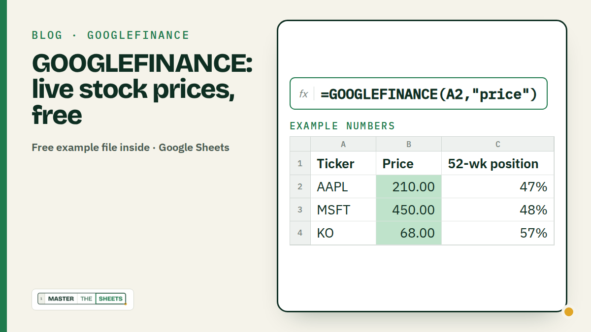
GOOGLEFINANCE pulls stock and currency data into Google Sheets for free: =GOOGLEFINANCE("NASDAQ:AAPL","price"). Change the second word to get the P/E, the market cap, the 52-week range or a whole price history.
I personally believe that if something cannot be modeled, tracked or calculated in a spreadsheet, that thing basically doesn't exist. However, managing my stock portfolio was very painful before I met =GOOGLEFINANCE.
The beauties of investing our money bring cases when on Day A our net worth increases by 15%, then on Day B it drops heavily (especially when big news hits the markets).
Honestly speaking, if you follow Warren Buffett's classic approach, keep most of your money in an index fund and leave it there for 40 years, the GOOGLEFINANCE function won't cause heavy breaths for you.
If you like doing your own modelling and working with live data, or simply want to know the trends, it will be a big deal. At least it was for me.
Here are some very cool things that it can do.
Before we start: GOOGLEFINANCE is Google Sheets only. Google says its quotes may be delayed by up to 20 minutes and are for information, not for trading. All prices in this article are example numbers to show how the formulas work, not real quotes, and nothing here is financial advice.
How GOOGLEFINANCE works
=GOOGLEFINANCE(ticker, [attribute], [start_date], [end_date|num_days], [interval])- ticker: the exchange and the symbol, like
"NASDAQ:AAPL"or"NYSE:KO", or a cell that holds it. - attribute (optional): what you want back. Leave it out and you get
"price". Useful ones:"price","changepct","pe","eps","marketcap","high52","low52","datadelay". - start_date (optional): add a date and GOOGLEFINANCE switches to history mode. The history attributes are
"open","close","high","low","volume"and"all". - end_date or num_days (optional): where the history stops, or how many days to fetch.
- interval (optional):
"DAILY"or"WEEKLY"(or 1 and 7).
Without a date you get one number in one cell. With a date you get a whole table that spills down, header row included.
1. Live prices for your watchlist
You follow a handful of stocks and you are tired of opening five tabs every morning. Type the tickers in column A.
| A: Ticker | B: Price (example) | C: Change % (example) | |
|---|---|---|---|
| 2 | NASDAQ:AAPL | 210.00 | 1.20 |
| 3 | NASDAQ:MSFT | 450.00 | -0.40 |
| 4 | NYSE:KO | 68.00 | 0.30 |
=GOOGLEFINANCE(A2,"price")          → 210.00 (example)
=GOOGLEFINANCE(A2,"changepct")      → 1.20 (example: +1.2% today)
Put the first formula in B2, the second in C2, and fill both down. Every row fetches its own ticker.
Pro tip: "changepct" comes back as a plain number, so 1.2 means +1.2%. Don't format it as a percentage or it shows 120%.
2. P/E and market cap: is it cheap or pricey?
Same tickers, one word changed.
| A: Ticker | B: P/E (example) | C: Market cap, $bn (example) | |
|---|---|---|---|
| 2 | NASDAQ:AAPL | 32.1 | 3,150 |
| 3 | NASDAQ:MSFT | 35.0 | 3,345 |
| 4 | NYSE:KO | 24.5 | 293 |
=GOOGLEFINANCE(A2,"pe")                         → 32.1 (example)
=GOOGLEFINANCE(A2,"marketcap")/1000000000       → 3,150 (example, in billions)
Market cap comes back in plain dollars, which is a lot of zeros. Dividing by 1,000,000,000 turns it into billions, so 3,150 means $3.15 trillion.
3. The 52-week range: where does the price sit?
A price on its own says little. Next to its 52-week low and high, it tells a story.
| A: Ticker | B: Price | C: 52-week low | D: 52-week high | E: Position | |
|---|---|---|---|---|---|
| 2 | NASDAQ:AAPL | 210.00 | 165.00 | 260.00 | 47% |
| 3 | NASDAQ:MSFT | 450.00 | 385.00 | 520.00 | 48% |
| 4 | NYSE:KO | 68.00 | 60.00 | 74.00 | 57% |
B, C and D are GOOGLEFINANCE formulas; the values shown are examples.
=GOOGLEFINANCE(A2,"low52")        → 165.00 (example)
=GOOGLEFINANCE(A2,"high52")       → 260.00 (example)
=(B2-C2)/(D2-C2)                  → 47%
0% means the price is sitting at its 52-week low, 100% means it is at the high. With the example numbers: (210 − 165) / (260 − 165) = 45 / 95 = 47%.
4. Price history and a trend line in one cell
Add dates and GOOGLEFINANCE hands you a whole table. Put the ticker in A2, the start date in B2 (1 Jul 2026) and the end date in C2 (31 Jul 2026).
| A: Ticker | B: Start | C: End | D: Trend | |
|---|---|---|---|---|
| 2 | NASDAQ:AAPL | 1 Jul 2026 | 31 Jul 2026 | (sparkline) |
The full table of daily closes, in A5:
=GOOGLEFINANCE(A2,"close",B2,C2,"DAILY")
→ Date                 Close
  1 Jul 2026 16:00     201.40 (example)
  2 Jul 2026 16:00     202.85 (example)
  …one row per trading day, 22 rows for July 2026
A tiny chart inside one cell, in D2:
=SPARKLINE(INDEX(GOOGLEFINANCE(A2,"close",B2,C2,"DAILY"),,2)) → a line of July's closesINDEX(…,,2) keeps only the second column (the closes), and SPARKLINE draws them. Swap B2 and C2 for TODAY()-90 and TODAY() and the trend is always the last 90 days.
Pro tip: the history table spills down, so give it empty rows below. If anything is in the way, you get a #REF! error instead of the table.
5. Currency conversion
Planning a trip, or paid in euros? GOOGLEFINANCE does exchange rates too.
| A: Item | B: Price in EUR | C: Price in USD | |
|---|---|---|---|
| 2 | Hotel, 3 nights | 480.00 | 528.00 (example) |
| 3 | Dinner | 65.00 | 71.50 (example) |
| 4 | Museum tickets | 24.00 | 26.40 (example) |
=GOOGLEFINANCE("CURRENCY:EURUSD")                → 1.10 (example rate)
=B2*GOOGLEFINANCE("CURRENCY:EURUSD")             → 528.00 (example)
The pattern is "CURRENCY:" followed by the two currency codes, from and to. Flip them ("CURRENCY:USDEUR") to go the other way. With the example rate, the whole €569 trip costs $625.90.
Pro tip: with a long list, fetch the rate once in its own cell and multiply by that cell. Fewer calls, faster sheet.
6. A mini portfolio that updates itself
Now put it all together: what you own, what you paid, what it is worth now.
| A: Ticker | B: Shares | C: Buy price | D: Price now (example) | E: Value | F: Gain % | |
|---|---|---|---|---|---|---|
| 2 | NASDAQ:AAPL | 10 | 150.00 | 210.00 | 2,100.00 | 40.0% |
| 3 | NASDAQ:MSFT | 5 | 300.00 | 450.00 | 2,250.00 | 50.0% |
| 4 | NYSE:KO | 20 | 55.00 | 68.00 | 1,360.00 | 23.6% |
=GOOGLEFINANCE(A2,"price")                        → 210.00 (example)
=B2*D2                                            → 2,100.00
=D2/C2-1                                          → 40.0%
=SUM(E2:E4)                                       → 5,710.00
=SUM(E2:E4)/SUMPRODUCT(B2:B4,C2:C4)-1             → 39.3%
SUMPRODUCT multiplies shares by buy price row by row and adds them up (your total cost, $4,100), so the last formula is the gain on the whole portfolio.
Common mistakes
- No exchange in the ticker.
"AAPL"usually works, but the same symbol can exist on several exchanges."NASDAQ:AAPL"always picks the right one. - Expecting live trading data. Quotes can be delayed by up to 20 minutes, and not every market is covered. Use it for tracking, not for timing trades.
- Blocking the spill. History formulas return a table. Leave empty cells below and to the right, or you get #REF!.
- Asking for a number that doesn't exist. Index funds and ETFs have no P/E, so
"pe"returns #N/A. Wrap it:=IFERROR(GOOGLEFINANCE(A2,"pe"),"-"). - Formatting changepct as a percentage. It is already in percent units: 1.2 means 1.2%.
FAQ
Is GOOGLEFINANCE free? Yes. It is a built-in Google Sheets function, and you only need a Google account.
How often does GOOGLEFINANCE update? The data refreshes while the sheet is open, but quotes can be delayed by up to 20 minutes. =GOOGLEFINANCE(A2,"datadelay") shows the delay for a ticker.
Does GOOGLEFINANCE work in Excel? No, it is Google Sheets only. In Excel 365, type the ticker, select it and choose Data > Stocks, then read fields like =A2.Price. For history, use =STOCKHISTORY(A2,B2,C2).
Can I use GOOGLEFINANCE for crypto or currencies? Currencies, yes: =GOOGLEFINANCE("CURRENCY:EURUSD"). Crypto coverage is limited, so check your ticker returns a value before you build on it.
Keep going
- Practise percentages and ROUND for free in the White Belt course: gain % is just a percentage change.
- Next read: QUERY: SQL inside Google Sheets. Sparklines (tiny charts in a cell) are coming soon.
Written by MasterTheSheets