Every spreadsheet error and how to fix it
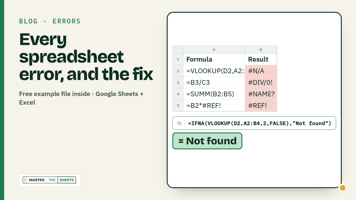
Every spreadsheet error is a clue. #N/A means a lookup can't find the value: check the spelling and hidden spaces, or add a fallback with =IFNA(VLOOKUP(D2, A2:B4, 2, FALSE), "Not found"). The other errors below each point at one specific cause, and each has a one-line fix.
I am a very chill guy. The bear from the famous meme is nothing compared to me in terms of being patient. But seeing a bunch of #REFs can drive me crazy in a fraction of a second.
If it is not your first rodeo with sheets, you will know stuff happens sometimes, but I can show you what the different error types mean, and what you can do to avoid and fix them.
How to read any error
- Read the name. Each error type has one main cause. The name alone tells you where to look.
- Hover over the cell. Google Sheets shows the full message when you hover (the red triangle in the corner). In Excel, click the small warning icon next to the cell.
- Follow the chain. An error spreads: if C2 is broken, every formula that uses C2 shows the same error. Fix the first one and the rest disappear.
- Fix the cause, then catch what's left. A fallback is fine for expected gaps, like a product that isn't in the list yet:
=IFNA(value, value_if_na)          catches only #N/A
=IFERROR(value, value_if_error)    catches every error
1. #N/A: the lookup can't find it
The value you look for isn't in the list. Or it is, but spelled differently. The classic sneaky one: a space at the end.
| A: Fruit | B: Price | C: | D: Find | |
|---|---|---|---|---|
| 2 | Apple | 1.20 | Pear (with a space after it) | |
| 3 | Pear | 0.90 | ||
| 4 | Plum | 1.50 |
=VLOOKUP(D2, A2:B4, 2, FALSE)                    → #N/A
=VLOOKUP(TRIM(D2), A2:B4, 2, FALSE)              → 0.90
TRIM removes the extra spaces. If the value really isn't there (say, Mango), give it a fallback instead of an ugly error:
=IFNA(VLOOKUP("Mango", A2:B4, 2, FALSE), "Not found")    → Not found
=XLOOKUP("Mango", A2:A4, B2:B4, "Not found")             → Not found
Pro tip: #N/A in a lookup is often useful. It tells you something is missing. Hide it only once you know why.
2. #REF!: the cell is gone
The formula points at a cell that no longer exists. Usually you deleted a row or column it used, and the reference turned into #REF! inside the formula.
| A: Item | B: Price | C: Qty | |
|---|---|---|---|
| 2 | Mug | 8.00 | 3 |
| 3 | Cap | 15.00 | 2 |
=B2*C2 gave 24. After someone deleted column C, it became:
=B2*#REF! → #REF!Fix: press Ctrl+Z (Cmd+Z on a Mac) straight away. Too late for that? Rewrite the reference by hand. In Excel you'll also get #REF! when you ask for a row outside a range: =INDEX(B2:B3, 3) → #REF!, because the range has only 2 rows. Google Sheets shows #NUM! for that one.
3. #VALUE!: text where a number should be
You're doing maths with something that isn't a number.
| A: Item | B: Price | C: Qty | |
|---|---|---|---|
| 2 | Mug | 8.00 | 3 pcs |
| 3 | Cap | 15.00 | 2 |
=B2*C2        → #VALUE!
=B3*C3        → 30
"3 pcs" is text. Fix: type 3 and move the unit into the header ("Qty, pcs"). For imported data you can't clean, strip the text inside the formula: =B2*VALUE(SUBSTITUTE(C2, " pcs", "")) → 24.
4. #DIV/0!: dividing by zero (or by nothing)
The cell you divide by is 0 or empty. An empty cell counts as 0.
| A: Rep | B: Sales | C: Calls | |
|---|---|---|---|
| 2 | Ana | 1,200 | 40 |
| 3 | Ben | 900 |
=B2/C2                               → 30
=B3/C3                               → #DIV/0!
=IF(C3=0, "No calls yet", B3/C3)     → No calls yet
Use "" instead of "No calls yet" if you'd rather see a blank until the number is filled in.
5. #NAME?: a typo
Spreadsheets don't recognise something you typed: a misspelled function, or text without quotes.
| A: Month | B: Sales | C: Paid | |
|---|---|---|---|
| 2 | Jan | 1,200 | Yes |
| 3 | Feb | 900 | No |
| 4 | Mar | 1,500 | Yes |
| 5 | Apr | 1,100 | Yes |
=SUMM(B2:B5)                  → #NAME?
=SUM(B2:B5)                   → 4,700
=COUNTIF(C2:C5, Yes)          → #NAME?
=COUNTIF(C2:C5, "Yes")        → 3
Fix: start typing the function and pick it from the list, so typos can't happen. Text always goes in double quotes.
6. #SPILL! (Excel) and #REF! (Google Sheets): no room for the results
Functions like FILTER, UNIQUE and SORT return several cells. If something is in the way, they can't spill.
| A: Name | B: Team | C: | D: Sales team | |
|---|---|---|---|---|
| 2 | Ana | Sales | (formula) | |
| 3 | Ben | Ops | old note | |
| 4 | Cleo | Sales | ||
| 5 | Dan | Ops |
=FILTER(A2:A5, B2:B5="Sales") → #SPILL! in Excel, #REF! in Google SheetsGoogle Sheets explains it on hover: "Array result was not expanded because it would overwrite data in D3." Fix: delete "old note" in D3 and the formula fills D2:D3 with Ana and Cleo.
7. #NUM!: maths that has no answer
The numbers are valid, but the calculation is impossible: the square root of a negative (=SQRT(-16)), a result too big to store, or a finance function that can't find an answer.
| A: Year | B: Cash flow | |
|---|---|---|
| 2 | 0 | $1,000 |
| 3 | 1 | $300 |
| 4 | 2 | $400 |
| 5 | 3 | $500 |
=IRR(B2:B5) → #NUM!IRR needs money going out and money coming in. The $1,000 investment is money out, so it needs a minus. Fix: type -1000 in B2, and =IRR(B2:B5) → 8.9%.
8. #ERROR!: Google Sheets can't read the formula
This one is Google Sheets only ("Formula parse error"). The formula breaks the grammar: a missing comma, an extra bracket, or semicolons in a sheet that expects commas. Excel won't even let you press Enter: it shows a "There's a problem with this formula" pop-up instead.
| A: Order | B: Amount | |
|---|---|---|
| 2 | 1001 | $80 |
| 3 | 1002 | $140 |
=IF(B2>100 "Big", "Small")        → #ERROR!
=IF(B2>100, "Big", "Small")       → Small
Fix: check the commas between arguments and count the brackets. Sheets colours each bracket pair, which helps.
9. Circular reference: the formula includes itself
A formula that uses its own cell, directly or through other cells, can never finish.
| A: Item | B: Cost | |
|---|---|---|
| 2 | Rent | $1,200 |
| 3 | Food | $450 |
| 4 | Fun | $150 |
| 5 | Total | (formula) |
=SUM(B2:B5) typed in B5 adds B5 to itself. Google Sheets shows #REF! ("Circular dependency detected"), Excel shows a warning and usually 0. Fix: stop the range one row above the total: =SUM(B2:B4) → $1,800.
Common mistakes
- Wrapping everything in IFERROR. It hides the real problems too: a typo in a range name returns your fallback forever. Fix the cause first, then catch only the errors you expect (IFNA for lookups).
- Fixing the last error in the chain. Find the first broken cell. Everything after it is just passing the error along.
- Numbers stored as text. Imported data often looks like numbers but isn't. It causes #VALUE!, #N/A in lookups and totals that are too small.
- Deleting columns in a finished sheet. Hide them instead, or check your totals right after deleting.
- Typing function names from memory. Pick them from the autocomplete list. #NAME? disappears for good.
FAQ
What does #N/A mean in Google Sheets and Excel? "Not available": a lookup like VLOOKUP, XLOOKUP or MATCH can't find the value. Check the spelling and hidden spaces (TRIM helps), or add a fallback with IFNA.
How do I hide #N/A errors? Wrap the lookup: =IFNA(VLOOKUP(D2, A2:B4, 2, FALSE), "") shows a blank instead. XLOOKUP has a built-in fallback as its fourth argument.
What's the difference between IFERROR and IFNA? IFNA only catches #N/A, so real mistakes (#REF!, #NAME?) still show. IFERROR catches everything. For lookups, IFNA is the safer choice.
Why do I get #REF! in Google Sheets when Excel shows #SPILL!? It's the same problem: a formula that returns several cells has no room. Google Sheets uses #REF! with the message "Array result was not expanded". Clear the cells in the way.
Keep going
- Practise IF, the function behind half the fixes above, for free in White Belt lesson 9.
- Next read: XLOOKUP vs VLOOKUP vs INDEX/MATCH and SUMIFS explained with 5 real examples.
Written by MasterTheSheets